yupsung Computer Science blog

1. Difference from other ML paradigms There is no supervisor, only a reward signal Feedback is delayed, not instantaneous Time really matters (sequential, non i.i.d. data) Agent’s actions affect the subsequent data it receives 2. Reward Reward $R_t$ : a scalar feedback signal Agent’s job is to maximize cumulative reward Reward hypothesis : all goals can be described by the maximization of expected cumulative reward 3. Sequential Decision Making Goal: select actions to maximize total future reward Reward may be delayed It may be better to sacrifice immediate reward to gain more long-term reward (greedy $\leftrightarrow$ optimal) 4. RL Agent Policy: agent’s behavior function Map from state to action Deterministic policy : $a = \pi (s) $ Stochastic policy : $\pi (a|s) = P[A_t = a | S_t = s] $ Value function: how good is each state and/or action Prediction of future reward. Evaluate the goodness/badness of states State-Value function $$v_{\pi}(s) = E_{\pi} [R_{t+1} + \gamma R_{t+2} +\gam

1. Ensemble Learning Set of models is integrated in some way to obtain the final prediction Homogeneous : It uses only one induction algorithm SVM1 + SVM2 + SVM3 ... Heterogeneous : It uses different induction algorithms SVM + DT + DNN + Bayesian ... Adds complexity Violation of Occam's Razor Decision boundary may become simpler Data manipulation : Changes the training set in order to obtain different models Manipulating the input features Sub-sampling from the training set Modeling process manipulation : Changes the induction algorithm Manipulating the parameter sets Manipulating the induction algorithm Combine Models Algebraic method : Average, Weighted Average, etc. Voting method : Majority Voting, Weighted Majority Voting, etc. Base Models : The base classifiers should be as accurate as possible and having diverse errors, while each classifier provides some positive evidences 2. Bagging (Bootstrap AGGregatING) Averaging the prediction over a collection of predictors generated f

1. Artificial Neural Network (인공신경망) Overfitting이 문제점이 되어 잘 사용되지 않았었음 2000년 초 해당 여러 문제가 해결되면서 많이 사용되기 시작 Training Decide input, output, hidden layer's number of node Find weight using training algorithm (Back-propagation algorithm) 2. Back-propagation algorithm Input layer에서 멀어질수록 Chain Rule에 의해서 Update되는 Weight의 양이 적어진다. Activation function 미분 가능한 함수! Sigmoid : 미분식 계산이 쉬움 $f^{\partial}(x) = f(x)(1-f(x))$ 3. Deep Neural Network Multiple hidden layers Vanishing gradient problem Sigmoid의 미분값은 0~0.25사이의 값 여러 layer를 update 하게 되면 계속 작아지는 문제가 발생 ReLU Layer-wise training Overfitting Collecting more data : consuming and expensive Data augmentation Dropout $\rightarrow$ Thinner model, ensemble, focus on more features(less idle node) Local minima Problem even with enough training data Start with multiple random points 4. Deep Neural Networks (cont.) 기존의 Machine Learning 방법의 경우 사람이 직접 feature를 선택(Hand crafted)하였고, 정보의 손실이 있어서 학습에 어려움이 있었다 반면 DNN은 학습을 통해 Data에서 적합한 feature를 추출하여 사용한다 유연하고 범용적으

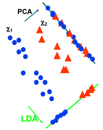
 1. Feature extraction / Dimensionality reduction Given data points in $d$ dimensions Convert them to data points in $k(<d)$  dimensions With minimal loss of information 2. Principal Component Analysis (PCA) Find k-dim projection that best preserves variance Process compute mean vector $\mu$ and covariance matrix $\Sigma$ of original data $$\Sigma = \frac{1}{N}\sum_{i=1}^N (x_i - \mu)(x_i-\mu)^T $$ Compute eigenvectors and eigenvalues of $\Sigma$ $$\Sigma v = \lambda v $$ Select largest $k$ eigenvalues (also eigenvectors) Project points onto subspace spanned by them $$y = A(x - \mu)$$ Eigenvector with largest eigenvalue captures the most variation among data $X$ We can compress the data by using the top few eigenvectors (principal components) Feature vector $y_k$'s are uncorrelated (orthogonal) 3. Linear Discriminant Analysis (LDA) PCA vs. LDA PCA does not consider "class" information LDA consider "class" information PCA maximizes projected total scatter LDA

 1. What is Clustering? Unsupervised learning Requires only data, no labels Detect patterns Useful when don't know what you're looking for Group together "similar" instances 2. Partition algorithms K-means Mixture of Gaussian Spectral clustering 3. Hierarchical algorithms Bottom up : Agglomerative Top-down : Divisive 4. K-means Clustering Objective : $$ \min_{\mu} \min_C \sum_{i=1}^k \sum_{x\in C_i} |x - \mu_i|^2$$ Initialize : Choose K points as cluster centers Alternate : (EM algorithm) Assignment step (Expectation) : Assign data points to closest cluster center $$Fix \;\mu,\; optimize\;C \\ \min_C \sum_{i=1}^k \sum_{x\in C_i} |x - \mu_i|^2 = \min_C \sum_{i=1}^n |x - \mu_{xi}|^2$$ Refitting step (Maximization) : Change the cluster center to the average of its assigned points $$Fix \;C,\; optimize\;\mu \\ \min_{\mu} \sum_{i=1}^k \sum_{x\in C_i} |x - \mu_i|^2$$ Stop : when no point assignment change 5. K-means Clustering (Properties) Guaranteed to converge in finite n

  1. 언제 사용하는가 ? Vector features Less than 20 attributes (Computational cost 가 높기 때문) Training data가 충분히 많을 때 2. 장점 Training이 매우 빠르다 복잡한 형태의 target function (decision boundary)도 학습 가능 원본 Data 정보 손실이 없다 3. 단점 Query 답변이 느리다 (거리 계산이 느림) 상관없는 attribute나 outlier에 취약하다 (Smoothing 이 없음) 4. Voronoi Diagram KNN 방법은 모든 training data를 저장 -> 많은 Memory 소모 Voronoi Diagram을 형성하여 Memory 소모량을 줄인다. Training time 증가 Test time 감소 5. Distance Metric Nearest를 결정하는 방법은 distance metric에 달려있음 Euclidean (L2) distance Manhattan / City-block (L1) distance 각 Dimension을 다르게 Scale 하는 Weighted 방법도 있음 그 외에도 다양... 6. Standardization (표준화) 원본(Raw) feature들을 새로운 Z-score로 변경 $$ z_{ij} = \frac{x_{ij} - \mu_j }{\sigma_j} $$ i번 sample의 j번 feature를 표준화 7. Efficient searching 효율적인 검색을 위해 데이터를 구조화 KD tree Choose dimension Choose pivot (median) Split data <repeat> 8. Choosing K Validation data가 없고, Train data만 있다면, N-fold cross validation을 사용 각 K에 대하여 K-NN을 Train, Test 진행 cross validation error가 가장 작은 K를 선택 (일반적으로 홀수) Tr

이번 글에서는 통계학에서 기본적으로 사용되는 용어, 개념들을 정리하였다. Sample space (표본공간) : The sample space $S$ is a set that contains all possible experimental outcomes. Experiment (실험) : Any process for which more than one outcome is possible. (Any process that generates data) Event (사건) : A subset of the sample space $S$ Random variable : A function that assigns real number to each element of sample space. $$Real\;numbers = f(Elements\;of\;the\;sample\;space)$$ 확률 변수의 종류 1. Discrete random variables (이산확률변수) : Outputs of a random variable are finite discrete (countable) values. (0, 1, 2, ...) 2. Continuous random variables (연속확률변수) : Outputs of a random variable are continuous (uncountable) values. Probability function ($f$) $$p = f(x)$$ $$x\;:\;Real\;numbers\;that\;the\;Random\;variables\;can\;take$$ $$0 \leq p \leq 1$$ $x$가 이산확률변수이면, $f$는 Probability mass function (p.m.f. : 확률질량함수) 이고 $x$가 연속확률변수이면, $f$는 Probability density function (p.d.f. : 확률밀도함수) 이다. Probability mass function (pmf : 확률 질량 함수) For a discr